4. System Overview

This section primarily describes the processing flow of the entire system.

Figure 4 illustrates the system architecture, showing that the system consists of four core modules:

1. Sequential-update ESIKF
2. Local map construction
3. LiDAR observation model
4. Visual observation model

Specifically, Module 1 deals with the ESIKF’s state prediction/update equations, while Modules 3 and 4 define the state observation equations of the ESIKF.

The processing flow is as follows: LiDAR points sampled asynchronously are merged to align with the camera’s sampling timestamps → Sequential updates are performed using ESIKF (first LiDAR, then camera). Both sensor modalities utilize a voxel map for management.

The LiDAR observation model performs frame-to-map point-to-plane residual calculations.

Visual map points within the current Field of View (FoV) are extracted from the voxel map using visible voxel queries and on-demand ray casting. Photometric errors (frame-to-map residuals, meaning the variation of photometric error between current and reference frames under pose perturbation ${}^G{T}_I$) are computed, enabling visual updates.

Local map maintenance: LiDAR-Inertial Odometry (LIO) updates geometric information of the voxel map, whereas Visual-Inertial Odometry (VIO) updates the current and reference image patches associated with the visual map points. (Updated reference image patches are further refined to obtain their normals in a separate thread.)

Sequential-update ESIKF

f readers are already familiar with ESIKF or the FAST-LIO system, this section can be skipped. However, for those unfamiliar, this section provides a step-by-step introduction to ESIKF.

This section introduces the mathematical models for state prediction and update, structured into four subsections: S

1. Notation and State Transition Model
2. Scan Recombination
3. Propagation (Forward and Backward Propagation)
4. Sequential Updates

Notation and State Transition Model

First, sensor coordinate frames are defined:

$$\begin{array}{r}I:\text{IMU frame}\\ G:\text{Global frame}\end{array}$$

(Note: Only IMU and global frames are defined here since the entire system state is IMU-centric. Observations from LiDAR and camera are transformed into the IMU frame.) Next, the discrete-time state transition equation is given by: $x_{i+1}=x_i⊞(\Delta tf(x_i,u_i,w_i))$

• $x_i$ is the state vector
• $u_i$ represents IMU observations
• $w_i$ is the process noise
• $\Delta t$ is the IMU sampling interval
• $f$ is the kinematic equation matrix (Note: When deriving the state-space equations, some methods begin by differentiating the kinematic equations in continuous time to obtain continuous-time state-space equations, which are then discretized. Discretization typically involves either Euler integration or midpoint integration. This process can be tedious, as continuous-time equations must first be obtained. A more convenient alternative is to directly discretize the kinematic equations and derive discrete-time state-space equations directly. Readers are encouraged to refer to additional blogs for further details on state-space equation derivations.)
• I have also translated + added more explainations here:
  • Data Fusion and Kalman Filter

Explanation of the $⊞$ operator:
Readers who have only read the FAST-LIVO2 paper may wonder what the $⊞$ symbol represents. In fact, it’s not complicated. This operator is explained clearly in the paper “FAST-LIO: A Fast, Robust LiDAR-Inertial Odometry Package by Tightly-Coupled Iterated Kalman Filter.” The operator arises primarily because rotation matrices $R\in SO(3)$ do not form a closed group under standard addition. Simply put, consider a coordinate frame F undergoing rotations $R_1^0$​ followed by $R_2^1$​, resulting in rotation $R_2^0$​. In this case, the relationship is $R_2^0\ne R_1^0+R_2^1$​, but rather $R_2^0=R_1^0{R}_2^1$​. Thus, the standard addition operator (+) becomes inappropriate for representing rotation increments. Hence, the $⊞$ operator is introduced to suitably represent “addition” operations involving both the rotation space $SO(3)$ and the Euclidean space ${\mathbb{R}}^n$.
(Note: This explanation is a simplified interpretation. To thoroughly understand addition and subtraction operations in $SO(3)$, readers are encouraged to further explore concepts related to manifolds and Rodrigues’ formula in sources like “Autonomous Driving and SLAM Technology in Robotics” or “14 Lectures on Visual SLAM” by Gao Xiang.)

Scan recombination

At the camera sampling timestamps, the high-frequency and sequentially sampled raw LiDAR points are segmented into different LiDAR scans. This ensures that camera and LiDAR data are synchronized at the same frequency (e.g., 10 Hz), enabling simultaneous state updates. Author’s explanatory note:
Let me share my initial understanding, followed by my updated comprehension after reading the code.

• Initial understanding:
  Having some prior knowledge about LiDAR, I initially thought scan recombination meant that LiDAR doesn’t capture all points simultaneously, but sequentially, point by point. For example, capturing a single frame of 24,000 points takes 100 ms, beginning at time $t_{k-1}$​ (the frame header time), and finishing at time $t_k$. These points are then merged into one frame. I assumed this recombination process was what the authors meant by “scan Recombination,” but I later realized this wasn’t correct.

• Understanding after code analysis:
  Because the camera’s trigger and exposure times aren’t perfectly stable, the exact LiDAR points corresponding to the camera’s capture time must be identified. Thus, each LiDAR point’s timestamp is evaluated individually: points timestamped before the camera’s capture time are classified as belonging to the current frame, while those after are attributed to the next frame. This process is actually what “scan recombination” refers to.

Additional note:
When reproducing results or reading the source code, readers might be confused by the additional 100 ms offset added to camera timestamps in the source code. Let me explain this based on my personal understanding:

• At time $t_{k-1}$​, the LiDAR begins capturing points, but initially, only the first point is captured.
• At time $t_k$​, the LiDAR completes the capture of an entire frame, and simultaneously, the camera captures an image.
• The camera driver then uses a shared timestamp file (a file created by Dr. Zheng himself to store the header timestamp of each point cloud frame) to assign the LiDAR’s frame header timestamp ($t_{k-1}$) to the camera frame as its timestamp.
• However, the camera data was actually captured at $t_k$, meaning there’s an inherent 100 ms offset between the original LiDAR timestamp and the assigned camera timestamp. This explains the additional 100 ms time offset present in the source code.

Propagation

Forward Propagation

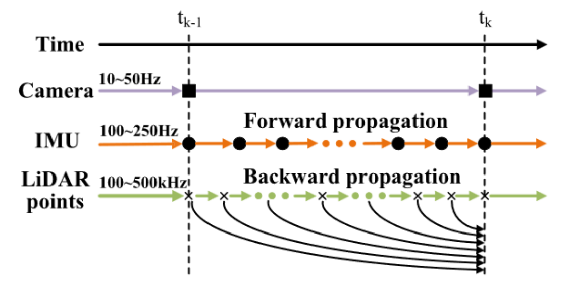Forward propagation is essentially the prediction step of an Extended Kalman Filter (EKF): during this prediction phase, the process noise $w_i$​ (which is unknown) is assumed to be zero. The system predicts states between times $t_{k-1}t$​ and $t_k$​ using IMU measurements. After EKF prediction, we obtain the predicted state vector and its corresponding covariance, which serves as the prior for the update step.

$$\begin{array}{r}{\hat{\mathbf{x}}}_{i+1}={\hat{x}}_i⊞(\Delta t\mathbf{f}({\hat{\mathbf{x}}}_i,{\mathbf{u}}_i),0)\\ \text{where }{{\hat{\mathbf{x}}}_0=\bar{\mathbf{x}}}_{k+1}\\ {\hat{\mathbf{P}}}_{\mathbf{i}+1}={\mathbf{F}}_{\widetilde{{\mathbf{x}}_{\mathbf{i}}}}{\hat{\mathbf{P}}}_{\mathbf{i}}{\mathbf{F}}_{{\tilde{\mathbf{x}}}_{\mathbf{i}}}^{\mathbf{T}}+{\mathbf{F}}_{{\mathbf{w}}_{\mathbf{i}}}{\mathbf{Q}}_{\mathbf{i}}{\mathbf{F}}_{{\mathbf{w}}_{\mathbf{i}}}^{\mathbf{T}}\\ \text{where }{{\hat{\mathbf{P}}}_0=\bar{\mathbf{P}}}_{k-1}\end{array}$$

Readers might be curious about how the state transition Jacobian matrices ${\mathbf{F}}_{\widetilde{x_i}}$ and ${\mathbf{F}}_{\widetilde{w_i}}$​​ are derived. Here, I recommend a blog, which clearly and simply explains the derivation and explicit forms of these state coefficient matrices.

Backward propagation

Backward propagation is essentially a correction for LiDAR motion distortion, ensuring that all points within a LiDAR scan are effectively observed at the same timestamp $t_k$.

What is Motion Distortion? As discussed in a Livox blog, motion distortion in LiDAR point clouds occurs because each point within a single LiDAR scan frame is captured under a slightly different coordinate system due to sensor movement. For instance, during a single frame interval, the LiDAR might be rapidly moving, thus capturing different points from different sensor poses. Consequently, points that should be collinear appear distorted because they reside in different coordinate frames:

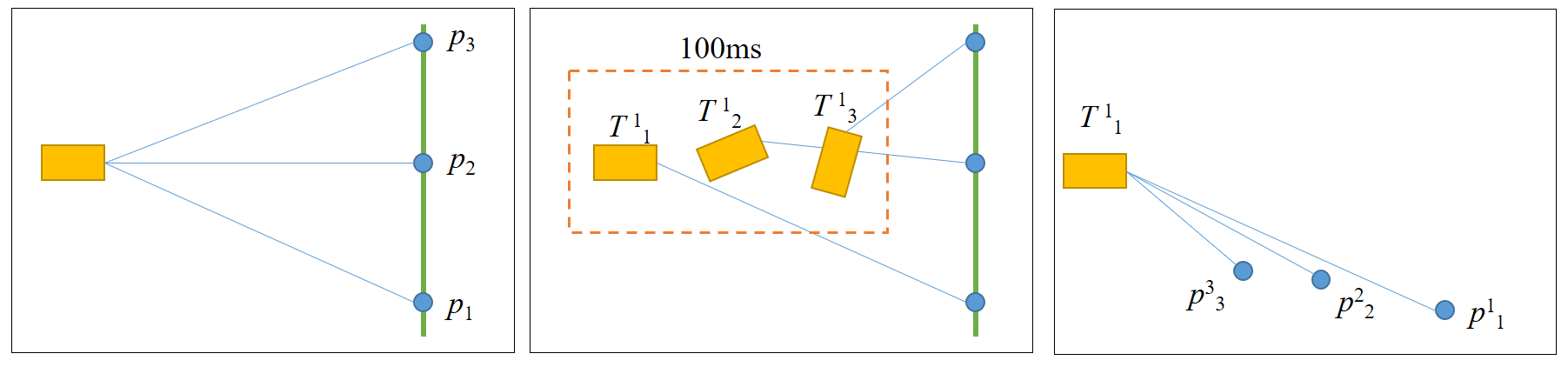figure 6: Motion distortion example

The solution: for each point between $t_{k-1}$ and $t_k$, determine the transformation matrix ${\check{T}}_{I_j}^{I_k}$ relative to timestamp $t_k$. (This was describe in the FAST-LIO paper)

Step-by-step Explanation:

• First, the state transition equation for backward propagation is established as:

$${\check{\mathbf{x}}}_{j-1}={\check{\mathbf{x}}}_j⊞(-\Delta t\mathbf{f}({\check{\mathbf{x}}}_{\mathbf{j}},{\mathbf{u}}_{\mathbf{j}},0))$$

• with the pose at $t_k$ as the initial reference pose. Here, $\Delta t$ is the time interval between LiDAR points.

• Next, LiDAR points between $t_{k-1}$ and $t_k$ are segmented according to IMU sampling intervals. A LiDAR point with timestamp ${\rho }_{j-1}$ belongs to some interval $[{\tau }_{i-1},{\tau }_i)$ defined by two consecutive IMU samples.
  • Example: A 10 Hz LiDAR (e.g., Livox Avia) generates 24,000 points per frame (100 ms), and a 200 Hz IMU generates 20 measurements in that same interval. Thus, multiple LiDAR points exist between any two IMU samples.
• Then, compute the transformation matrices at each timestamp relative to timestamp $t_k$:
  1. Rotation Matrix at timestamp $j$ relative to $t_k$, ${}^{I_k}{\check{R}}_{I_j}$

$${}^{I_k}{\hat{\mathbf{R}}}_{I_{j-1}}={}^{I_K}{\hat{\mathbf{R}}}_{I_j}\cdot \text{Exp}\left(({\hat{\mathbf{b}}}_{{\omega }_k}-{\omega }_{m_{i-1}})\Delta t\right),{}^{I_k}{R}_{I_m}=I$$

• Note: Within interval $[{\tau }_{i-1},{\tau }_i)$, the angular velocity is assumed constant, approximated by the IMU angular velocity at ${\tau }_{i-1}$. The bias is fixed at the prior at $t_k$.

2. Velocity at timestamp $j$ relative to $t_k$ ${}^{I_k}{\check{v}}_{I_j}$:

$$\begin{array}{rl}{}^{I_k}{\check{\mathbf{v}}}_{I_{j-1}}& ={}^{I_k}{\check{\mathbf{v}}}_{I_j}-{}^{I_k}{\check{\mathbf{R}}}_{I_j}\left({\mathbf{a}}_{m_{i-1}}-{\hat{\mathbf{b}}}_{a_k}\right)\Delta t-{}^{I_k}{\hat{\mathbf{g}}}_k\Delta t,\\ \text{s.f.}{}^{I_k}{\check{\mathbf{v}}}_{I_m}& ={}^G{\hat{\mathbf{R}}}_{I_k}^T{}^G{\hat{\mathbf{v}}}_{I_k},{}^{I_k}{\hat{\mathbf{g}}}_k={}^G{\hat{\mathbf{R}}}_{I_k}^T{}^G{\hat{\mathbf{g}}}_k.\end{array}$$

• Acceleration within this interval is assumed constant, equal to the IMU acceleration at ${\tau }_{i-1}$. Acceleration biases and gravity are assumed fixed at their prior values at $t_k$.

3. Translation at timestamp $j$ relative to $t_k$: ${}^{I_k}{\check{p}}_{I_j}$

$$\begin{array}{rl}{}^{I_k}{\check{\mathbf{p}}}_{I_{j-1}}& ={}^{I_k}{\check{\mathbf{p}}}_{I_j}-{}^{I_k}{\check{\mathbf{v}}}_{I_j}\Delta t,\\ \text{s.f.}{}^{I_k}{\check{\mathbf{p}}}_{I_m}& =0.\end{array}$$

• Using computed velocities and accelerations, translation $p_{I_j}^{I_k}$ is calculated accordingly.

Finally, transforming each LiDAR point yields the corrected (undistorted) points at timestamp $t_k$:

$${}^{L_k}{\mathbf{p}}_{f_j}={\left({}^I{T}_L\right)}^{-1}{}^{I_k}{T}_{I_j}{}^{L_j}{p}_{f_j}$$