Data Fusion and Kalman Filter

translated from: https://blog.csdn.net/qq_42731705/article/details/129420739

Intro example

when given different measurement devices, how can we obtain the diameter of a coin?

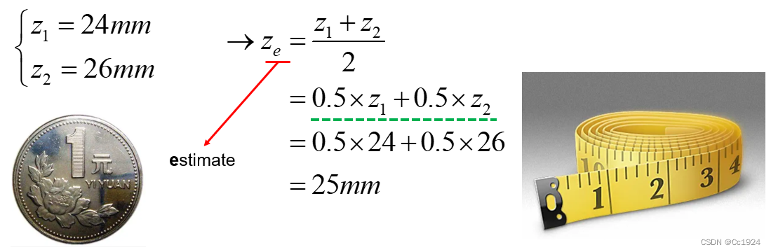
Test 1: Measuring tape

we can use the measuring tape to measure the diameter of the radius twice, measurements $z_1$ and $z_2$. Taking the average gives the estimate

$$z_e=25\text{mm}$$

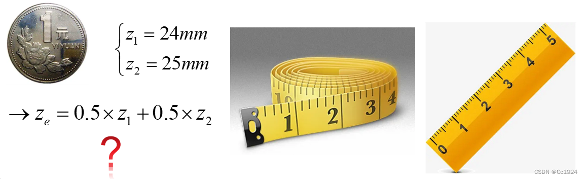
Test 2: measuring tape + ruler of different resolutions

To obtain the estimate $z_e$ would we still average the measurements?

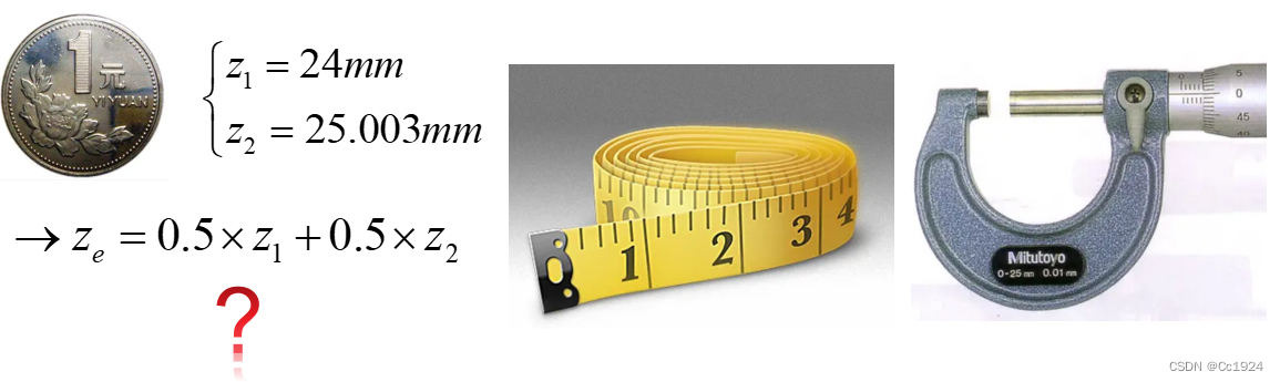
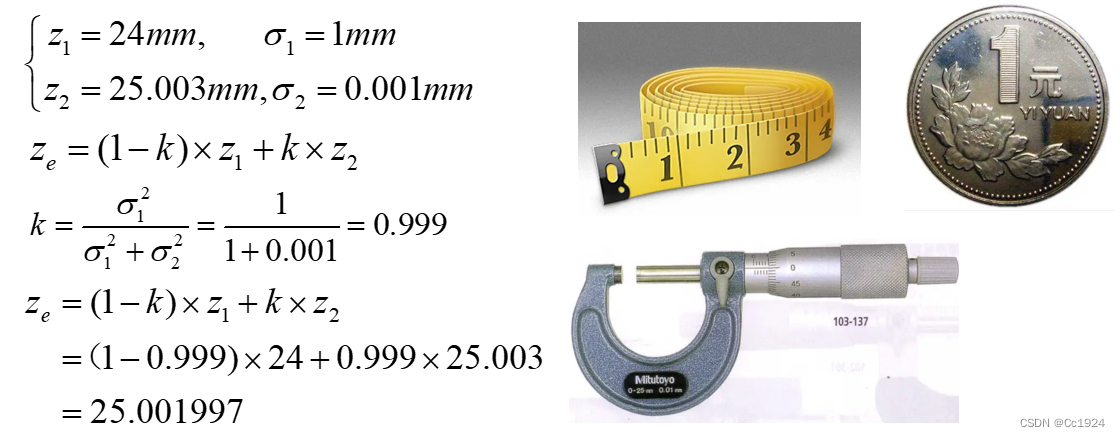
Test 3: measuring tape and micro meter

In this case, would we still take one measurement each and take the average? Even though the micrometer’s resolution is much higher than the measuring tape? (1mm vs 0.001mm)

Intuition: No

Obviously, since sensor precisions differ, we can no longer simply average the readings from different sensors. Because, neglecting systematic error, a micrometer’s measurement is clearly more accurate than that of a tape measure.

So how can we obtain the best estimate of the coin’s diameter from measurements made by different sensors? That’s where the data‐fusion methods described later come in!

Data fusion

What does Data fusion do?

Using different sensors to achieve the best estimate of the system. In the example above, it would be to use different sensors (measuring devices) to give a best estimation of the coin’s diameter.

Prerequisite for Data Fusion — Uncertainty

No sensor is perfectly accurate, nor is there any measurement process that is completely error‑free. In other words, every single measurement comes with some uncertainty. When we ignore systematic errors, a higher‑precision sensor will have a smaller measurement uncertainty. For example, in the case above, the measurement uncertainty of the micrometer is much smaller than that of the tape measure.

In statistics, uncertainty is expressed in terms of standard deviation, variance, and the covariance matrix. Clearly, in the previous example, when computing a weighted average of measurements from different sensors, we should take each sensor’s uncertainty into account: the smaller the uncertainty, the larger the weight its measurement should carry, because it is more accurate. 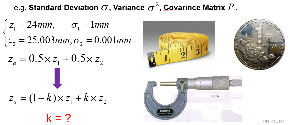If we know the standard deviation of the measurements produced by each sensor, we should be able to derive a weight $k$ in order to assign different weights (importance/trustworthiness) to each measurement.

Result of Data Fusion: The Statistically Optimal Estimate

Every measurement carries uncertainty, so from a statistical standpoint our measurement is a random variable, and the final estimate of the system state is also a random variable. The optimal data‐fusion result, therefore, should minimize variance; for a multivariate random variable this means achieving the smallest possible trace of the covariance matrix.

Hence, when we derive the weighted average of the measurements from different sensors below, our goal is to choose weights so that the resulting weighted average has the minimum variance.

• Optimal Estimation: fusion result with the minimum uncertainty, i.e minimum $\sigma ,{\sigma }^2,P$

Example

Suppose we have measurements:

$$\begin{array}{rl}{z}_1=& 24\text{mm},{\sigma }_1=1\text{mm}\\ z_2=& 25.003\text{mm},{\sigma }_2=0.001\text{mm}\end{array}$$

goal: to find value $k$ such that the estimation has minimal uncertainty

$$\begin{array}{r}{z}_e=(1-k)z_1+k{z}_2\end{array}$$

ans: recall that

$$\begin{array}{rl}{\sigma }_{z_e}^2=& Var[(1-l)z_1+k{z}_2]\\ =& Var[(1-k)z_1]+Var[k{z}_2]\\ =& (1-k{)}^{2}Var[z_1]+k^{2}Var[z_2]\end{array}$$

due to properties of variance, we have

$$\begin{array}{rl}{\sigma }_{z_e}^2=& (1-k{)}^2{\sigma }_1^2+k^2{\sigma }_2^2\end{array}$$

since ${\sigma }_1$ and ${\sigma }_2$ are constants in this case, we can differentiate ${\sigma }_{z_e}$ with respect to $k$ to find the minima.

$$\begin{array}{rl}\frac{d{\sigma }_{z_e}^2}{dk}=& -2(1-k){\sigma }_1^2+2k{\sigma }_2^2\\ 0=& -2(1-k){\sigma }_1^2+2k{\sigma }_2^2\\ k=& \frac{{\sigma }_1^2}{{\sigma }_1^2+{\sigma }_2^2}\end{array}$$

The result is easy to interpret in two scenarios:

• If ${\sigma }_1^2$ is very large, then $k$ tends toward 1, and the fused result approaches $z_2$. This makes sense: measurement 1 has a large variance (i.e., is less accurate), so we lean on measurement 2.
• If ${\sigma }_2^2$ is very large, then $k$ tends toward 0, and the fused result approaches $z_1$. The reasoning is analogous. Plugging our derived formula into the previous example of measuring the coin’s diameter with a tape measure and a micrometer, we find that the final fused estimate lies very close to the micrometer’s reading, which is exactly the desirable outcome.

State Space Representation

In robotic state‑estimation problems, it’s not simply a matter of taking two sensor measurements and fusing them. Instead, one usually builds a motion model of the system that lets us predict its state. When new sensor data arrives, we update that prediction based on the measurements, yielding a more accurate estimate of the system state.

This process is precisely the system’s state‑space formulation. In the Kalman Filter, it’s broken into two parts: the state equation and the observation (measurement) equation.

State equation

We construct a mathematical model of the system’s physics. For example, in SLAM, if we assume the robot travels at constant velocity or under constant acceleration, then our models become the constant‑velocity model or the constant‑acceleration model, respectively.

In short, the state equation is something we calculate or derive. Given the system state at the previous time step, we use the state equation to compute the current system state, this constitutes our prediction.

Another point to note, as mentioned in the Data Fusion section, is that both measurements and our mathematical model carry uncertainty. For instance, our model may be imperfect, so the state equation is subject to noise. In the Kalman Filter, we assume this noise is Gaussian, an essential premise for deriving the Kalman Gain.

$$x_k=A{x}_{k-1}+B{u}_{k-1}+w_{k-1},$$

• $A$: state‑transition matrix
• $B$: control‑input matrix
• $u_{k-1}$: control vector
• $w_{k-1}$: process noise, assumed to be drawn from multivariate normal distribution with zero‑mean and covariance $Q$

$A$: State‑Transition Matrix

• What it is: A matrix that encodes your system’s built‑in dynamics—how the state moves forward in time if there were no external inputs or noise.
• Role in the equation: In

$$x_k=A{x}_{k-1}+B{u}_{k-1}+w_{k-1},$$

the term $A{x}_{k-1}$ is your prediction of the new state $x_k$ based sData Fusion and Kalman Filterolely on the old one.

• Intuition:
• If your state is just a 1D position and you assume it doesn’t change by itself, $A=1$.
• If your state is $\left[\begin{array}{c}\text{position}\\ \text{velocity}\end{array}\right]$ under a constant‑velocity model, then with timestep $\Delta t$:

$$A=\left[\begin{array}{cc}1& \Delta t\\ 0& 1\end{array}\right],$$

because (from kinematics)

$${\text{pos}}_k={\text{pos}}_{k-1}+\Delta t{\text{vel}}_{k-1},$$

and (from constant velocity assumption)

$${\text{vel}}_k={\text{vel}}_{k-1}.$$

• Details: suppose our state $x_i=\left[\begin{array}{c}{p}_i\\ v_i\end{array}\right]$ at some timestep $i$, then

$$\begin{array}{rl}{x}_k=& A\cdot x_{k-1}\\ =& \left[\begin{array}{cc}1& \Delta t\\ 0& 1\end{array}\right]\cdot \left[\begin{array}{c}{p}_{k-1}\\ v_{k-1}\end{array}\right]\\ =& \left[\begin{array}{c}1\cdot p_{k-1}+\Delta t\cdot v_{k-1}\\ 0\cdot p_{k-1}+1\cdot v_{k-1}\end{array}\right]\\ =& \left[\begin{array}{c}{p}_{k-1}+\Delta t{v}_{k-1}\\ v_{k-1}\end{array}\right]\end{array}$$

which matches above.

Q: So we have to derive $A$ ourselves every time we need to apply a kalman filter?

$B$:Control‑Input Matrix

• What it is: A matrix that describes how your known inputs or controls $u$ (e.g. commanded acceleration, wheel‑encoder speeds) push the state forward.
• Role in the equation: In

$$x_k=A{x}_{k-1}+B{u}_{k-1}+w_{k-1},$$

the term $B{u}_{k-1}$ injects the effect of your control actions.

• Intuition:
• If your control $u$ is a direct velocity command in a 1D position‑only model, you might set

$$A=1,B=\Delta t,$$

so that $Bu=\Delta t\cdot (\text{velocity})$ updates your position.

• In the 2‑state $[\text{pos};\text{vel}]$ constant‑acceleration model, if $u$ is acceleration $a$, you’d choose

$$B=\left[\begin{array}{c}\frac{1}{2}\Delta t^2\\ \Delta t\end{array}\right],$$

because

$$\text{pos increment}=\frac{1}{2}a\Delta t^2,\text{vel increment}=a\Delta t.$$

Summary

• $A$ tells you “where the system would go on its own.”
• $B$ tells you “how external commands or controls nudge it.”

Observation Equation

This is just like our earlier example of measuring the coin’s diameter: it describes how we observe the system’s state. In SLAM, however, the observation is often indirect and mediated by an observation model. For instance, in visual‑inertial odometry (VIO) we want to estimate the system’s 6 DOF pose, but what the camera actually gives us are pixel coordinates of feature points, not the pose itself. Those pixel measurements are related to the 6 DOF state through the camera’s projection model. In other words, the projection model ties the actual observed pixel values to the true pose, and that relationship is our observation equation.

In summary, although the observation equation doesn’t measure the system state directly, it indirectly measures it via the observation model, so it still constitutes a measurement of the state.

Likewise, observations are noisy: feature‐point locations may be imprecise, and the projection model itself might not be perfect. Therefore we add Gaussian noise to the observation equation, and it must be Gaussian, because that assumption is necessary for deriving the Kalman Gain.

Intuition: At each time step $k$, you get a new sensor reading $z_k$. The Kalman‐filter observation equation

$$z_k=H_k{x}_k+v_k$$

says that:

1. $x_k$ is the true system state at time $k$ (e.g.\ position/velocity, 6‑DOF pose, etc.).

2. $H_k$ is the observation matrix (or model) that tells you how the state maps into whatever your sensor actually measures.

• If your state is $\left[\begin{array}{c}\text{pos}\\ \text{vel}\end{array}\right]$ but your sensor only reads position, then

$$H=\left[\begin{array}{cc}1& 0\end{array}\right]$$

so that $z_k=[10]\left[\begin{array}{c}{\text{pos}}_k\\ {\text{vel}}_k\end{array}\right]={\text{pos}}_k$.

• In a camera case, $H_k$ would be the projection from 3‑D pose into pixel coordinates.

3. $v_k$ is the measurement noise, capturing all the ways your sensor might err (electronic noise, quantization, feature‐extraction error, etc.). We model it as

$$v_k\sim \mathcal{N}(0,R_k),$$

meaning zero‑mean Gaussian with covariance $R_k$. The size and shape of $R_k$ encode how much trust you place in that sensor—and whether different measurements are correlated.

Example of System State-Space Equations

Suppose we have a small car equipped with:

• A single‑line laser rangefinder that measures its distance from the starting point, and
• A wheel encoder that measures the wheel’s speed. Our goal is to estimate the car’s state, so we can write its state-space model like so:

State Equation

We want to arrive at something in this form

$$x_k=A{x}_{k-1}+B{u}_{k-1}+w_{k-1}$$

Start: Recall the discrete‐time kinematic update:

$$x_k=x_{k-1}+(\text{true velocity})\times \Delta t$$

but we only measure velocity with noise:

• $v_{k-1}$ the measured velocity at time $k-1$,
• $w_{k-1}$ the zero‐mean process noise on that velocity.

$$v_{\text{true}}=v_{k-1}-w_{k-1}.$$

Plug that into the kinematic step:

$$x_k=x_{k-1}+v_{\text{true}}\Delta t=x_{k-1}+(v_{k-1}-w_{k-1})\Delta t.$$

After distributing the $\Delta t$,

$$x_k=x_{k-1}+v_{k-1}\Delta t-w_{k-1}\Delta t$$

We can then match it to

$$\begin{array}{rl}{x}_k& =A{x}_{k-1}+B{u}_{k-1}-W{w}_{k-1},\end{array}$$

• since $x_{k-1}=A{x}_{k-1}$, it follows that $A=1$
• likewise $B=\Delta t$, and $W=-\Delta t$
• and $w_{k-1}\sim \mathcal{N}(0,Q).$

Note: You always start with your true (possibly nonlinear) update, then group all deterministic terms into $Ax+Bu$ and bundle every approximation or uncertainty into the additive “noise” term $Ww$.

Observation Equation

$$z_k=H{x}_k+v_k$$

In our running example the sensor reads position directly, so

$$z_k=x_k+v_k,v_k\sim \mathcal{N}(0,R),$$

and hence $H=1$.

Note: “starting point” for your observation equation always comes from your sensor model. In other words, from how the sensor actually measures the thing you care about. In general you write:

$$z_k=h\left(x_k\right)+v_k,$$

where:

• $h(x_k)$ is the true (possibly nonlinear) mapping from state → sensor reading,
• $v_k$ is the additive measurement noise.

Summary

• $A=1$: With no inputs and no noise you’d stay in place.
• $B=\Delta t$: Converts encoder‐measured velocity into position change.
• $w$: Process‐noise on the motion model (e.g. wheel slip) enters through $W=-\Delta t$.
• $H=1$: The laser directly measures position.
• $v$: Measurement‐noise on the laser reading.

Note: In the setup above, we put the wheel‑encoder measurement into the state equation (as the control input $u$) and the laser measurement into the observation equation. You might wonder: aren’t both sensors just making observations? Why not treat the wheel encoder like any other measurement? In fact, these two choices are mathematically equivalent.

• Wheel encoder in the state equation:
  • You model its noise as part of the process noise $w$ acting on the control input $u$.
• Wheel encoder in the observation equation:
  • You set $u=0$ in the state equation and propagate velocity purely via the previous state, then treat the encoder reading as a second measurement $z$ that constrains the velocity in the observation equation.

Both formulations impose the same information on the filter; they simply differ in whether you view the encoder as an “input” or a “measurement.”

Kalman Filter

What does a Kalman filter do?

Despite its name, the Kalman Filter isn’t really a “filter” in the signal‐processing sense but a state estimator. Its job is to combine your state equation

$$x_k=A{x}_{k-1}+B{u}_{k-1}+w_{k-1},w_{k-1}\sim \mathcal{N}(0,Q)$$

and your observation equation

$$z_k=H{x}_k+v_k,v_k\sim \mathcal{N}(0,R)$$

to produce the statistically optimal estimate of the true state $x_k$ (i.e.\ minimum‑variance unbiased).

Two Key Assumptions

1. Linearity: Both the state‐transition model and the observation model must be linear in the state variable—hence the constant matrices $A$ and $H$.
2. Gaussian Noise: Both the process noise $w$ and the measurement noise $v$ are assumed zero‑mean Gaussian. Only under these two conditions does the algebraic derivation of the Kalman Gain guarantee that the fused estimate achieves the minimum possible error covariance in a purely statistical sense.

Kalman Fitler Intuition

Because we have two noisy estimates of the same state

• ${\hat{x}}_k$ from the model (state equation), and
• $x_k^{(m)}$ from the sensor (observation equation) we fuse them exactly as we did when averaging two coin‐diameter measurements, choosing weights to minimize the final variance.

Derivation

1. State equation (the “calculated” or predicted estimate)

$$x_k=A{x}_{k-1}+B{u}_{k-1}+w_{k-1}.$$

Since $w_{k-1}$ is zero‐mean, we replace it by its expectation (zero) when forming the prior estimate:

$${\hat{x}}_k=A{x}_{k-1}+B{u}_{k-1}.$$

2. Observation equation (the “measured” estimate)

$$z_k=H{x}_k+v_k.$$

Likewise, $v_k$ has zero mean, so to get a direct state estimate from the measurement we momentarily ignore $v_k$ and invert $H$:

$$x_k^{(m)}=H^{-1}{z}_k.$$

Why “zero out” the noises and invert $H$?

• Zero‐mean noise: In reality $w$ and $v$ aren’t zero, but we only know their statistics. If we had the actual noise values we wouldn’t need a filter, we’d just plug them in. Hence in the derivation we substitute the mean of each noise term (zero).

• Inverting $H$: This step is purely for intuition, to view the sensor’s reading as a “direct” state estimate. The final Kalman‐filter update never explicitly computes $H^{-1}$; instead it uses a gain matrix that blends prediction and measurement optimally. Applying the data‑fusion idea, we simply form a weighted average of the predicted state and the measured state, like this:

$$\{\begin{array}{l}{z}_1=24\text{ mm},{\sigma }_1=1\text{ mm}\\ z_2=25.003\text{ mm},{\sigma }_2=0.001\text{ mm}\end{array}$$ $$z_e=0.5z_1+0.5z_2⟹z_e=(1-k)z_1+k{z}_2$$ $${\sigma }_e^2=\mathrm{Var}[(1-k)z_1+k{z}_2]=(1-k{)}^2{\sigma }_1^2+k^2{\sigma }_2^2$$ $$\frac{d{\sigma }_e^2}{dk}=-2(1-k){\sigma }_1^2+2k{\sigma }_2^2=0⟹k=\frac{{\sigma }_1^2}{{\sigma }_1^2+{\sigma }_2^2}$$ $${\tilde{x}}_k=(I-G){\hat{x}}_k+G{x}_k^m$$

Kalman Filter Task: Using the State equation and Observation equation to get the optimal state estimation

1. State equation (calculated):

$${\hat{x}}_k=A{x}_{k-1}+B{u}_{k-1}$$

2. Observation equation (measured):

$$z_k=H{x}_k^m⟹x_k^m=H^{-1}{z}_k$$

By algebraically manipulating that weighted‑average formula, eliminating the need to explicitly invert $H$:

We start with the weighted-average fusion:

$${\tilde{x}}_k=(I-G){\hat{x}}_k+G{x}_k^m$$

• ${\hat{x}}_k$ is your prior (predicted) state,
• $x_k^m$ is your measured state (i.e.\ $H^{-1}{z}_k$),
• $G$ is the matrix of weights you’ll choose (analogous to the scalar $k$ in the coin example).
• $I-G$ is the complementary weight on the prior.

We then substitute in the direct measurement form, since $x_k^m=H^{-1}{z}_k$,

$${\tilde{x}}_k=(I-G){\hat{x}}_k+G(H^{-1}{z}_k).$$

Regroup to expose the “innovation” $(z_k-H{\hat{x}}_k)$. Add and subtract $G{H}^{-1}H{\hat{x}}_k$ inside:

$$\begin{array}{rl}{\tilde{x}}_k& =(I-G){\hat{x}}_k+G{H}^{-1}{z}_k\\ & ={\hat{x}}_k-G{\hat{x}}_k+G{H}^{-1}{z}_k\\ & ={\hat{x}}_k+G(H^{-1}{z}_k-{\hat{x}}_k)\end{array}$$

Notice that $H^{-1}{z}_k-{\hat{x}}_k=H^{-1}(z_k-H{\hat{x}}_k).$

$$={\hat{x}}_k+G{H}^{-1}(z_k-H{\hat{x}}_k).$$

The vector $(z_k-H{\hat{x}}_k)$ is called the innovation or measurement residual—it’s how much the actual sensor reading $z_k$ differs from what your prediction $H{\hat{x}}_k$ would imply.

Define the Kalman gain $K$, let

$$K=G{H}^{-1}.$$

Then the update becomes the classic Kalman‐filter form:

$$\boxed{{\tilde{x}}_k={\hat{x}}_k+K(z_k-H{\hat{x}}_k).}$$

• ${\hat{x}}_k$ is your prior,
• $z_k-H{\hat{x}}_k$ is the innovation,
• $K$ is the gain that determines how much of that innovation you trust.

Summary

1. You start by imagining “let’s just weight‐average” prediction vs. (inverted) measurement.
2. Realize that weighting the direct measurement $H^{-1}{z}_k$ is equivalent to adding a correction proportional to the difference between what you saw $(z_k)$ and what you expected $(H{\hat{x}}_k)$.
3. That proportionality matrix is exactly the Kalman gain $K$.

Choosing $K$ to minimize the posterior covariance is what makes the Kalman filter “optimal” in the minimum‑variance sense.

By applying the data‐fusion idea, our ultimate goal is to find a suitable weighting coefficient so that the final weighted‐average result has the smallest variance. For a multivariate random variable, this means minimizing the trace of its covariance matrix. As shown below: 2. Posterior update (weighted‐average fusion)

$${\tilde{x}}_k={\hat{x}}_k+K(z_k-H{\hat{x}}_k).$$

• ${\hat{x}}_k$: prior (predicted) state
• $z_k$: new measurement
• $H$: observation matrix
• $K$: gain matrix (to be determined)

1. Posterior covariance Denote the resulting covariance of ${\tilde{x}}_k$ by ${\tilde{P}}_k$.
2. Optimization criterion $$K=\underset{K}{\mathrm{argmin}}\mathrm{tr}\left({\tilde{P}}_k\right),$$ i.e. choose $K$ to make the trace of the posterior covariance as small as possible.
3. Covariances in play
   • Prediction covariance: ${\hat{P}}_k=A{\tilde{P}}_{k-1}{A}^T+Q$
   • Measurement covariance: $R$ Putting it all together, the Kalman Gain $K$ is the weight that minimizes $\mathrm{tr}({\tilde{P}}_k)$.

Note:

• The covariance of the predicted state, ${\hat{P}}_k$, is obtained by propagating the previous covariance through the state equation.
• The covariance for the observation equation, since we haven’t transformed measurements from observation space into state space (i.e. we didn’t compute any pseudo‑inverse of $H$), is simply the observation noise covariance $R$.

Prediction covariance derivation: We have the true state update

$$x_k=A{x}_{k-1}+B{u}_{k-1}+w_{k-1},w_{k-1}\sim \mathcal{N}(0,Q),$$

and the prior (predicted) estimate

$${\hat{x}}_k=A{\tilde{x}}_{k-1}+B{u}_{k-1}.$$

Define the prediction error

$${\epsilon }_k=x_k-{\hat{x}}_k.$$

Propagate the error, substitute $x_k$ from the state‐equation:

$$\begin{array}{rl}{\epsilon }_k& =(A{x}_{k-1}+B{u}_{k-1}+w_{k-1})-(A{\tilde{x}}_{k-1}+B{u}_{k-1})\\ & =A(x_{k-1}-{\tilde{x}}_{k-1})+w_{k-1}\\ & =A{\epsilon }_{k-1}+w_{k-1}.\end{array}$$

Compute the prior covariance: By definition: In general, for any random column‐vector $y$ we define its covariance as

$$\mathrm{Cov}(y)=\mathbb{E}[(y-\mathbb{E}[y])(y-\mathbb{E}[y]{)}^T].$$

Since

• We let ${\epsilon }_k=x_k-{\hat{x}}_k$ be the prediction error.
• Under the usual Kalman assumptions (zero‐mean process and measurement noise, and an unbiased filter), that error itself has zero mean, i.e.\ $\mathbb{E}[{\epsilon }_k]=0$. Hence its covariance simplifies to

$$\mathrm{Cov}({\epsilon }_k)=\mathbb{E}\left[{\epsilon }_k{\epsilon }_k^T\right],$$

Thus we arrive at:

$${\hat{P}}_k=\mathrm{Cov}\left({\epsilon }_k\right)=\mathbb{E}\left[{\epsilon }_k{\epsilon }_k^T\right].$$

Using ${\epsilon }_k=A{\epsilon }_{k-1}+w_{k-1}$ and the facts that ${\epsilon }_{k-1}$ and $w_{k-1}$ are uncorrelated, and $\mathrm{Cov}(w_{k-1})=Q$, we get

$$\begin{array}{rl}{\hat{P}}_k& =\mathbb{E}[(A{\epsilon }_{k-1}+w_{k-1})(A{\epsilon }_{k-1}+w_{k-1}{)}^T]\\ & =A\mathbb{E}[{\epsilon }_{k-1}{\epsilon }_{k-1}^T]A^T+\mathbb{E}[w_{k-1}{w}_{k-1}^T]\\ & =A{\tilde{P}}_{k-1}{A}^T+Q.\end{array}$$

Measurement covariance derivation Your observation equation is

$$z_k=H{x}_k+v_k,v_k\sim \mathcal{N}(0,R).$$

Here, $R$ is defined to be the covariance of the measurement noise $v_k$. Thus any time you fuse or weight in a new measurement, the amount of uncertainty that measurement brings in is exactly $R$.

Kalman Gain

is very complicated lol, for full derivation: https://www.bilibili.com/video/BV1hC4y1b7K7/?spm_id_from=333.788&vd_source=1363e3b30e51ca9984f82492949f865b or https://blog.csdn.net/qq_42731705/article/details/129423983

For now we just use the result:

$$\boxed{K=\frac{{\hat{P}}_k{H}^T}{H{\hat{P}}_k{H}^T+R}}⟺K={\hat{P}}_k{H}^T(H{\hat{P}}_k{H}^T+R{)}^{-1}.$$

This choice of $K$ is exactly the weight matrix that minimizes the trace of the posterior covariance. 2. Posterior Covariance Update

$${\tilde{P}}_k=(I-KH){\hat{P}}_k.$$

Together, these two equations complete the Kalman‐filter “measurement‐update” step:

• You compute $K$ from your prior covariance ${\hat{P}}_k$, the observation model $H$, and the measurement‐noise covariance $R$.
• You then update the covariance to ${\tilde{P}}_k$, which is guaranteed to be the minimum‐variance (i.e. minimum trace) posterior under the linear‑Gaussian assumptions.

Summary

State‐Equation Prediction: Using the previous time step’s state and the system’s state‐space equation, we compute a prediction of the current state. At the same time, we update the covariance matrix of that predicted state: Definitions of all symbols assume $x_k\in {\mathbb{R}}^n$, $u_k\in {\mathbb{R}}^m$, $z_k\in {\mathbb{R}}^p$

(1) Prior estimation

$${\hat{x}}_k=A{\tilde{x}}_{k-1}+B{u}_{k-1},$$

• ${\hat{x}}_k\in {\mathbb{R}}^n$: prior (predicted) state estimate at time $k$.
• $A\in {\mathbb{R}}^{n\times n}$: state‑transition matrix.
• ${\tilde{x}}_{k-1}\in {\mathbb{R}}^n$: posterior state estimate at time $k-1$.
• $B\in {\mathbb{R}}^{n\times m}$: control‑input matrix.
• $u_{k-1}\in {\mathbb{R}}^m$: control (input) vector at time $k-1$.

(2) Prior covariance

$${\hat{P}}_k=A{\tilde{P}}_{k-1}{A}^T+Q.$$

• ${\hat{P}}_k\in {\mathbb{R}}^{n\times n}$: prior error‐covariance at time $k$.
• ${\tilde{P}}_{k-1}\in {\mathbb{R}}^{n\times n}$: posterior covariance at time $k-1$.
• $Q\in {\mathbb{R}}^{n\times n}$: process‐noise covariance.

Observation‐Equation Update: First compute the Kalman Gain $K$. Then treat $K$ as the weight to fuse the predicted state with the sensor’s measurement, yielding the optimal state estimate: (3) Kalman Gain

$$K=\frac{{\hat{P}}_k{H}^T}{H{\hat{P}}_k{H}^T+R}⟺K={\hat{P}}_k{H}^T(H{\hat{P}}_k{H}^T+R{)}^{-1}$$

• $K\in {\mathbb{R}}^{n\times p}$: Kalman‐gain matrix.
• ${\hat{P}}_k\in {\mathbb{R}}^{n\times n}$: prior covariance (from (2)).
• $H\in {\mathbb{R}}^{p\times n}$: observation matrix.
• $H^T\in {\mathbb{R}}^{n\times p}$: transpose of $H$.
• $R\in {\mathbb{R}}^{p\times p}$: measurement‐noise covariance.

(4) Posteriori (updated) state estimate

$${\tilde{x}}_k={\hat{x}}_k+K(z_k-H{\hat{x}}_k)$$

• ${\tilde{x}}_k$: Posterior (updated) estimate of the state at time $k$.
• ${\hat{x}}_k$: Prior estimate (from Eq 1).
• $K$: Kalman gain (from Eq 3).
• $z_k$: Measurement vector at time $k$.
• $H$: Observation matrix.

(5) Posteriori covariance

$${\tilde{P}}_k=(I-KH){\hat{P}}_k$$

• ${\tilde{x}}_k\in {\mathbb{R}}^n$: posterior (updated) state estimate at time $k$.
• ${\hat{x}}_k\in {\mathbb{R}}^n$: prior state estimate (from (1)).
• $K\in {\mathbb{R}}^{n\times p}$: Kalman gain (from (3)).
• $z_k\in {\mathbb{R}}^p$: measurement vector.
• $H\in {\mathbb{R}}^{p\times n}$: observation matrix. Notice that the prediction is in units of the system state, while the measurement is in the sensor’s native units. Therefore the Kalman Gain $K$ carries physical units, it has the same units as $H^{-1}$.